Getting Started

This section provides an overview on how to setup and use Py\(\small\mathbb{SOFE}\).

Installation

Please note that Py\(\small\mathbb{SOFE}\) has been developped and tested under Linux and Python 2.7.

A prerequisite for the installation of Py\(\small\mathbb{SOFE}\) is that you already have installed Python on your computer as well as the modules setuptools and pip. If this is not the case, please follow this guide to do so.

If you have troubles installing Py\(\small\mathbb{SOFE}\), please don’t hesitate to contact me.

PyPI

Py\(\small\mathbb{SOFE}\) is hosted at the Python Packaging Index so the easiest way of installing it would be by running:

$ pip install pysofe

in a terminal, provided that you have installed the Python module pip

Source

If you would like to install Py\(\small\mathbb{SOFE}\) from the source files please download the latest release from here. After the download is complete open the archive and change directory into the extracted folder. Then run the following command:

$ python setup.py install

Usage

This sections is intended to provide a minimalistic worked example to show the basic usage of Py\(\small\mathbb{SOFE}\).

Consider the linear Poisson equation on the unit square in 2D with homogeneous Dirichlet boundary conditions

\[\begin{align*} a\Delta u(x) &= f(x) &&\text{ in }\Omega=(0,1)^2 \\ u(x) &= 0 &&\text{ on }\partial\Omega \end{align*}\]

with the constant coefficient \(a\) and the right hand site \(f \in L^2(\Omega)\). To keep things simple let \(a = 1\) and define \(f(x) = x_0^2 - x_1^2\) where \(x = (x_0,x_1)\in\Omega\subset\mathbb{R}^2\).

First, we create the mesh that discretizes the spatial domain \(\Omega\) of our problem. To do so we import the predefined class UnitSquareMesh and instantiate a mesh with \(100\) nodes on each axis

>>> from pysofe import UnitSquareMesh
>>> mesh = UnitSquareMesh(100, 100)

Then, we create the reference element that provides the basis functions. We will use linear basis functions on triangles, implemented in the class P1 which takes the spatial dimension of our problem as an argument

>>> from pysofe import P1
>>> element = P1(dimension=2)

Next, we create the function space in which we look for a solution. We do this by creating an instance of the FESpace class that brings together the mesh and reference element

>>> from pysofe import FESpace
>>> fe_space = FESpace(mesh, element)

For the formulation of our problem we also need to specify boundary conditions the solution should comply with. This part takes a bit more effort than the previous steps.

The first thing to do for this is to define a function specifying the boundary where the conditions should hold. Py\(\small\mathbb{SOFE}\) expects a function that decides for a given array of points which of them lie on the boundary. In our case the boundary points are determined by their \(x_0\) and \(x_1\) coordinate which are equal to \(0\) or \(1\) on the boundary of the unit square

>>> from numpy import logical_or as or_
>>> def dirichlet_domain(x):
...     x0_is_0_or_1 = or_(x[0] == 0., x[0] == 1.)
...     x1_is_0_or_1 = or_(x[1] == 0., x[1] == 1.)
...     return or_(x0_is_0_or_1, x1_is_0_or_1)

Then, since we want to impose a Dirichlet boundary condition, we need to define the function that the solution of our problem should be equal to on the boundary. In the simple case of a homogeneous boundary condition it suffices to define this function as a constant

>>> g = 0.

Now, we can create the boundary condition implemented in the DirichletBC class and pass the arguments defined above

>>> from pysofe import DirichletBC
>>> dirichlet_bc = DirichletBC(fe_space, dirichlet_domain, g)

What remains is to define the actual boundary value problem. Therefore, we will use the predefined Poisson class. But first we need to define the parameters for this class which are the factor \(a\) and the right hand site function \(f\). Since we set the constant factor \(a\) equal to \(1\) we can simply do so in the code as well

>>> a = 1.

and we define the right hand site as

>>> def f(x):
...     return x[0]*x[0] - x[1]*x[1]

So, now we have all things we need to create the object that represent our boundary value problem

>>> from pysofe import Poisson
>>> pde = Poisson(fe_space, a, f, dirichlet_bc)

Finally, to solve it we call

>>> u = pde.solve()

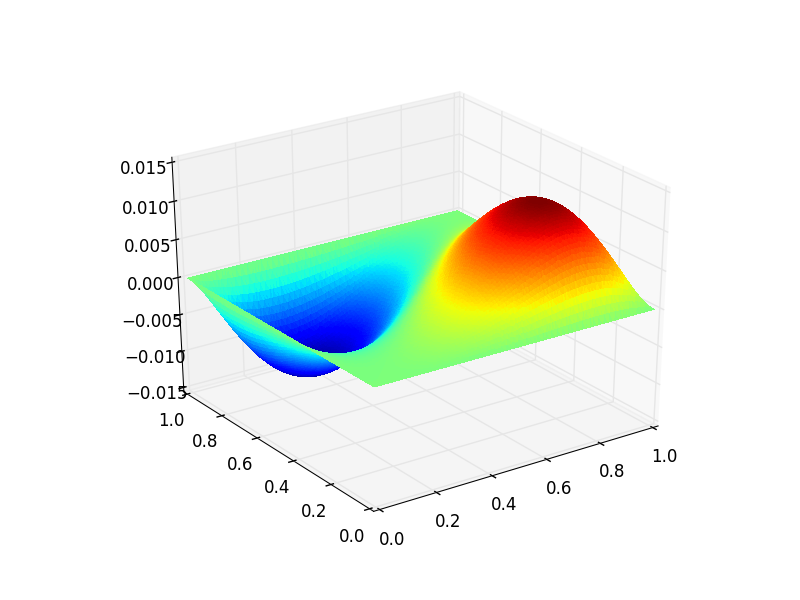
which returns a callable function object that represents our approximate solution and can be visualized with

>>> import pysofe
>>> pysofe.show(u)

which should produce the following graphics.